This post focuses on how to calculate simple summary statistics

What goes in your .csv and what goes in your R script

Before I get into how to summarize your data, I wanted to have a brief discussion on what should go into your R script versus what should go into your .csv file. One of the major reasons to code is to have transparency in your analysis. Therefore, your .csv file should have all of your raw data; nothing should be calculated even if it is easy. For example, let’s say you have a file with community data: each column is one species and each row is data from one site. In your file you have two different species of snails, but you only care about the total number of snails across all species. In excel, it is very easy to sum across these columns and add a new column for snails, but try to resist. It is way better to put this simple equation in R so that everyone can see what you did and why. Of course, there are always exceptions, but try as best as you can to include only raw data in your .csv file and all your calculations in your R code.

Summary statistics

Today, we are going to talk about how to summarize your data using the plyr package. If you do not already have this package installed on your computer then make sure to install it using the following code.

install.packages('plyr')

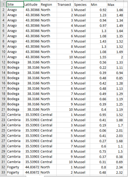
We will be using data from Piper to learn how to calculate various summary stats. Piper is looking at the vertical distribution patterns of different intertidal organisms. She has data on the lower and upper range limits of multiple species (tide heights) from 10 transects per site across 14 sites. Here is how her .csv file is set-up.

First, let’s set-up our scripts just like we learned in last weeks lesson.

#################################################### 
# Script to summarize Piper's vertical data        #
# Created by Nyssa                                 #
# created on 1/23/2017                             #
####################################################

## clear workspace---------
rm(list=ls())

## set working directory------
setwd(getwd())

# load libraries------------------
library(plyr)

## Load Data-------------
Data<-read.csv('Data/Vertical.csv')

## Data analysis-----------------

# clean the data--------------
# check the data
head(Data)
tail(Data)

You will see that piper has two data columns: one for the lower range limit within a transect (Min) and one for the upper limit (Max). She is also interested in the overall tidal range of each species, which is calculated as Max - Min.

# we create a new column in the dataframe for range
Data$Range<-Data$Max - Data$Min

#check that it worked
head(Data)

Next, let’s take her site names, which are factors, and order them by latitude so that when we make plots they will be ordered from south to north instead of alphabetically. Last week, you will remember that we manually told R what order we wanted Lauren’s microhabitats to be in. Here, Piper has latitude data associated with each site which makes it very easy to automate this step. Below, I used the function order() to produce the indices of the variable of interest in decending (or ascending, if you want) order. So, if I put order(Data$Latitude) then I will get values of 1 to the number of rows, where 1 is the southern most latitude and the highest number is the northern most. Then, I used the function unique() because the latitude and site names are repeated multiple times.

# order the sites by latitude
Data$Site <- ordered(Data$Site, levels =unique(Data$Site[order(Data$Latitude)]) )

Now, we will calculate means, SE, mins, and maxs of the different variables of interest across sites and species. To do this, we will use the ddply function from the plyr packages. To see the list of arguments required type ?ddply into R.

## take the average tide height by species (mussels and barnacles) and site
Data.summary<-ddply(Data, c("Site","Species"), summarize,
                 mean.Range = mean(Range, na.rm=TRUE), # this is saying to take the mean range and ignore missing data if there is any
                 N = sum(!is.na(Range)), # how many samples do you have (code says what is not a missing value and sum the counts)
                 Abund.SE = sd(Range, na.rm = TRUE)/sqrt(N), # this is the standard error,
                 mean.min = mean(Min, na.rm=TRUE), # average lower limit across transects per site and species
                 mean.max = mean(Max, na.rm=TRUE), # average upper limit
                 min.Min = min(Min, na.rm=TRUE), # minimum tide height across all transects within a site
                 max.Max = max(Max, na.rm=TRUE), # max height across all transects
                 lat=mean(Latitude) # add a column of latitude
)

There is now a new data frame with all the summary stats called Data.summary. Now, try to calculate summary stats for Region and Species on your own.

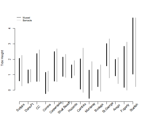
We can now use this summary data to make a simple plot to visualize species overlap within the intertidal across sites. The plot below is a bit more complicated than last week. If you are unsure of what the different arguments mean remember that you can also use the help file by putting a ? in front of the function name.

# plot the ranges
png(filename = 'Output/PiperRange.png',width = 580, height = 480) #create a .png file
# create an empty plot without axes so that we can add in layers one by one
plot(NULL, type="n", axes=F, xlab="", ylab='Tide Height', ylim=c(min(Data$Min),max(Data$Max, na.rm=TRUE)), xlim=c(1,14), cex.axis=0.5, cex.lab=1)
# vertical lines from min to max tide height for mussels
arrows(1:14,Data.summary$min.Min[Data.summary$Species=='Mussel'],
       1:14,Data.summary$max.Max[Data.summary$Species=='Mussel'], length=0, angle=90, code=3, lwd=3)
# vertical lines for barnacles next to the mussel lines
arrows(1:14+0.3,Data.summary$min.Min[Data.summary$Species=='Barnacle'],
       1:14+0.3,Data.summary$max.Max[Data.summary$Species=='Barnacle'], length=0, angle=90, code=3, lwd=3, col='grey')
#add back axes
# x-axis
axis(1, 1:14, labels = FALSE,lwd.ticks = .5, tck=-0.03 )
# y-axis
axis(2, cex.axis=1)
# add site names at a 45 degree angle instead of the numbers 1:14 on the x-axis
text(1:14, par("usr")[3]-0.2,  labels = unique(Data.summary$Site), srt = 45, pos = 1, xpd = TRUE)
# add a legend
legend('topleft',c('Mussel','Barnacle'),lty=1, col=c('black','grey'), cex=0.75, bty='n')
# close the graphics device
dev.off()

This code makes a plot that looks like this: