This post focuses on how to write a a random intercept, random slope and intercept, and nested mixed effects model in the nlme package.

#Work in progress

Mixed Effects Models

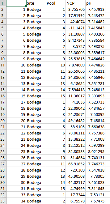
Today, we will use some of my biogeochemistry data. I am going to use mixed effects models to test the relationship between net community production (NCP) and pH while accounting for within and between site-level variability. I collected 12 replicate samples at 15 different tide pools within 4 different sites. Here is what the data look like:

Using the above data set we will run a random intercept model to account for site-level variability, a random intercept and random slope model accounting for site-level variability, and a nested random slope model accounting for site and pool within site-level variability.

Random Intercept Model

lme stands for linear mixed effects model. Inside the brackets is read as y (your dependent variable) is a function of x (your independent variable) and is called a formula (exactly the same as last week). RInt is the factor that you want your data to vary by. It is your random effect. This code can also be used for multiple x parameters.

Here, x1, x2, and x3 are three different independent variables.

Let’s test if there is a significant linear relationship between NCP and pH while allowing the intercept to vary by Site.

Here is what the code looks this:

m<-lme(pH ~  NCP, random = ~1|Site, data=d2)

Here, my dataframe is called d2 and I named the model output m

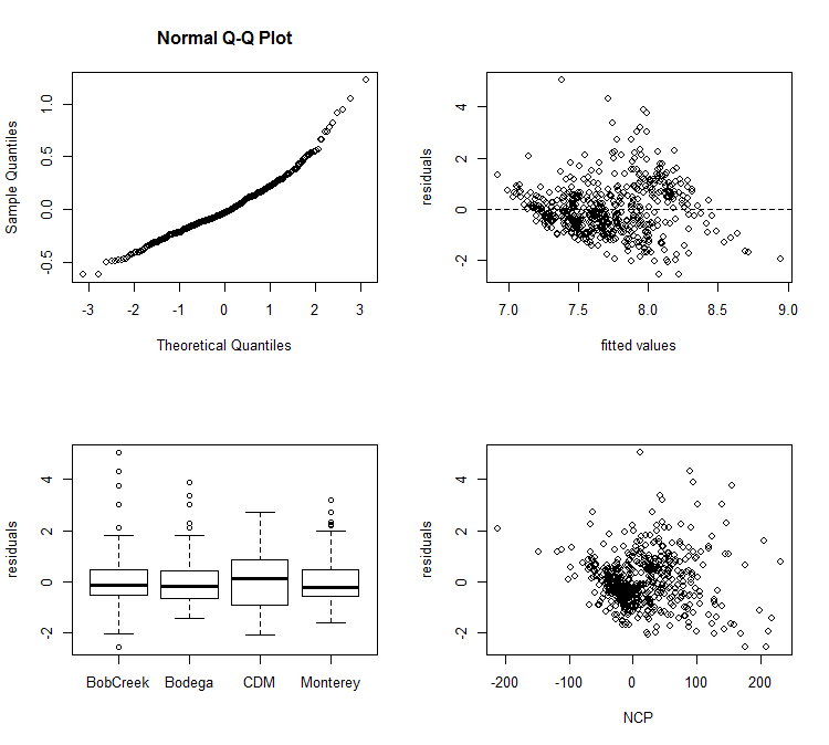
The first step in forming any model is to check that we have met all of the assumptions of a linear mixed effects model. Do we have normal residuals, are our data independent, and do we have equal variances across our different groups? We can visually check all these assumptions with the following code:

# test assumptions----------------------
# test fit of the residuals.  There should be no patterns
par(mfrow=c(2,2)) # make the subplots
qqnorm(resid(m))
E2<-resid(m, type = "normalized") # extract normalized residuals
F2<-fitted(m) # extract the fitted data
plot(F2, E2, xlab = "fitted values", ylab = "residuals") # plot the relationship
abline(h = 0, lty = 2) # add a flat line at zerp

# test for homogeneity of variances
boxplot(E2~d2$Site, ylab = "residuals")

# check for independence. There should be no pattern
plot(E2~d2$NCP, ylab = 'residuals', xlab = "NCP")

Here, is what those plots look like:

When we see that everything looks good then we can view our results. The ANOVA and summary tables have exactly the same code as the lm models. However, in the summary table you will also see the variance due to the random effect of site.

# look at the anova table and summary statistics
anova(m)
summary(m)

To pull out the different coefficients, we use the fixef() function for the fixed effects and the ranef() function for the random effects.

## pull out the random and fixed effects
ranef(m) # random
fixef(m) # fixed

Lastly, we will want to plot the data. First, let’s plot the raw data with a different color for every site.

# Plot the data
par(mfrow=c(1,1)) # only plot the data in one subplot
plot(d2$NCP, d2$pH, col = d2$Site, xlab = 'NCP', ylab = 'pH')

Now, let’s plot the best fit lines. There are two types of best fit lines: one for the whole model (fitted across sites) and one highlighting the random intercepts(fitted between sites). We can extract these two levels of heirarchy in the fitted() function that we discussed last week by setting level = 0 (full model) and level = 1 (between sites).

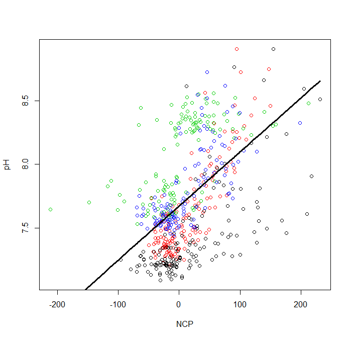
# extract the fitted values to make a best fit line
F0<-fitted(m, level = 0) # fitted across sites
F1<-fitted(m, level = 1) # fitted between sites

Now, one kind of annoying thing is that the x and y values need to be ordered to plot a straight line. So we need to add one more step before plotting the fitted lines.

# we need to put the data in order so that we can actually create a line
I<-order(d2$NCP)
# plot the best line for the entire model
lines(d2$NCP[I], F0[I],  lwd = 3, xlim=range(d2$NCP), ylim = range(d2$pH))

Now, we can look at the best fit line for the entire model.

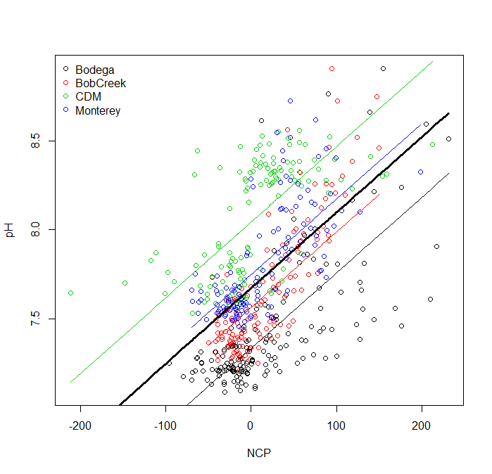
Next, let’s add the best fit lines for the between sites model. To do this we will need to use a for loop where we will loop over the 4 sites.

# create an array of unique sites
Sites<-unique(d2$Site)

# plot the best line with the random intercepts
for (i in 1:length(Sites)){
  x1<-d2$NCP[d2$Site==Sites[i]] # x value at site i
  y1<-F1[d2$Site==Sites[i]] # y value at site i
  ind<-order(x1) # reorder the data
  lines(x1[ind],y1[ind], col = Sites[i]) # make the plot
}
# add a legend
legend("topleft",legend= Sites, col=c(1,2,3,4), pch=21, bty="n")

Here, is what the final plot looks like: